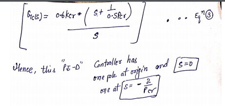
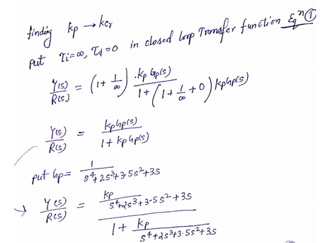

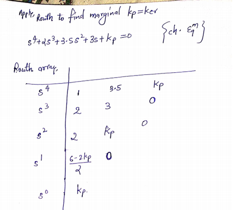
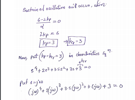
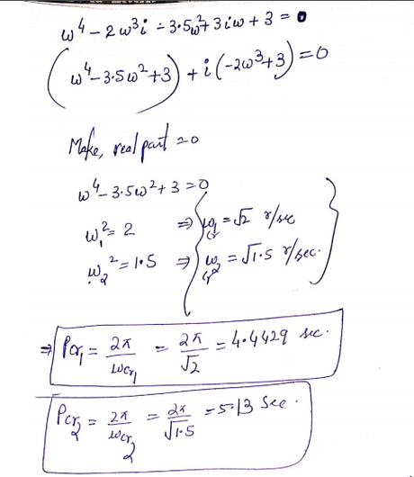
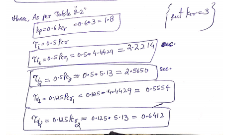
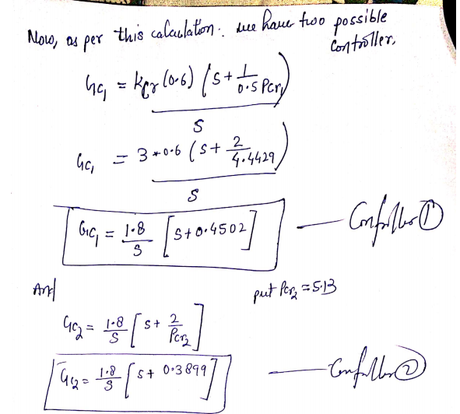
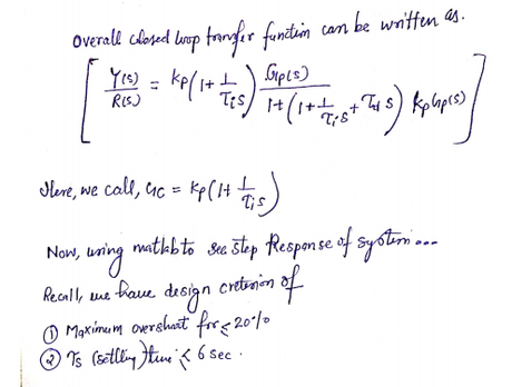
%type the following command in matlab to get two closed loop transfer function and there
%step response to check the overshoot and settling time criterion
clc
clear all
kp=3;
Ti1=2.2214;
Ti2=2.5650;
Td1=0.5554;
Td2=0.6412′
Kcr=kp;
s = tf(‘s’);
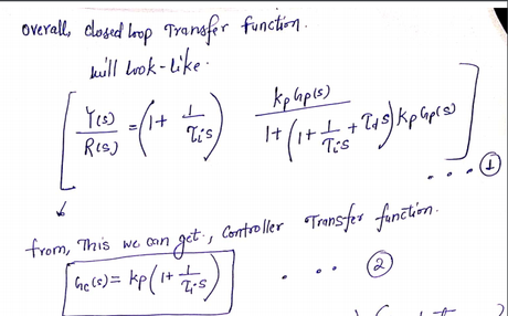
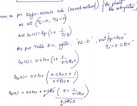
Gc1=kp*(1+(1/(Ti1*s)))
Gc2=kp*(1+(1/(Ti1*s)))
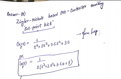
Gp=1/(s^4+(2*s^3)+(3.5*s^2)+(3*s))
%closed loop transfer function
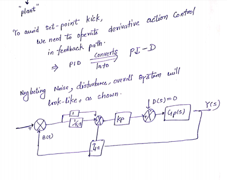
Den1=(1+(1/(Ti1*s))+(Td1*s))
Den2=(1+(1/(Ti2*s))+(Td2*s))
T1=Gc1*(Gp/(1+(Den1*Gp*kp)))
T2=Gc1*(Gp/(1+(Den2*Gp*kp)))
step(T1)
stepinfo(T1)
grid
figure
step(T2)
stepinfo(T2)
%In command window we get
Continuous-time transfer function.
T1 =
8.882 s^6 + 21.76 s^5 + 39.09 s^4 + 40.64 s^3 + 12 s^2
——————————————————————————————————
4.935 s^10 + 19.74 s^9 + 54.28 s^8 + 103.6 s^7 + 138.4 s^6 + 142.7 s^5 + 98.3 s^4 + 40.64 s^3 + 12 s^2
Continuous-time transfer function.
T2 =
10.26 s^6 + 25.13 s^5 + 45.13 s^4 + 46.93 s^3 + 13.85 s^2
——————————————————————————————————-
5.698 s^10 + 22.79 s^9 + 62.68 s^8 + 120.5 s^7 + 161.6 s^6 + 167.2 s^5 + 114.9 s^4 + 44.76 s^3 + 12 s^2
Continuous-time transfer function.
system_info_T1 =
RiseTime: 1.3153
SettlingTime: 18.8828
SettlingMin: 0.7410
SettlingMax: 1.8293
Overshoot: 82.9269
Undershoot: 0
Peak: 1.8293
PeakTime: 4.3556
system_info_T2 =
RiseTime: 1.4426
SettlingTime: 21.3147
SettlingMin: 0.9923
SettlingMax: 1.8059
Overshoot: 56.4002
Undershoot: 0
Peak: 1.8059
PeakTime: 4.3987
See step responses in figure window for T1 and T2 transfer function
For T1 Step response is
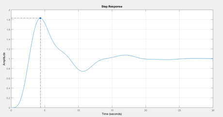
system_info_T1 =
RiseTime: 1.3153
SettlingTime: 18.8828
SettlingMin: 0.7410
SettlingMax: 1.8293
Overshoot: 82.9269
Undershoot: 0
Peak: 1.8293
PeakTime: 4.3556
For T2 we got
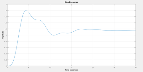
system_info_T2 =
RiseTime: 1.4426
SettlingTime: 21.3147
SettlingMin: 0.9923
SettlingMax: 1.8059
Overshoot: 56.4002
Undershoot: 0
Peak: 1.8059
PeakTime: 4.3987
We will work with T1 and T2 both, closed loop transfer functions to meet design criteria of:-
- Less than 20 percent overshoot
- Less 6 seconds settling time
%New line of Code to meet design criteria by ziegler method2
% to meet design criteria we need to tune the parameters of Kp, Ti , Td
%keep on varying the values until we get to the desired level of overshoot
% and Settling time
clc
clear all
clc
clear all
kcr=2.0199;
kp=0.6*kcr;
Ti1=7.2214;
Ti2=10.13087;
Td1=0.5554;
Td2=0.0000006777777777;
s = tf(‘s’);
Gc1=kp*(1+(1/(Ti1*s)))
Gc2=kp*(1+(1/(Ti1*s)))
Gp=1/(s^4+(2*s^3)+(3.5*s^2)+(3*s))
%closed loop transfer function
Den1=(1+(1/(Ti1*s))+(Td1*s))
Den2=(1+(1/(Ti2*s))+(Td2*s))
T1=Gc1*(Gp/(1+(Den1*Gp*kp)))
T2=Gc1*(Gp/(1+(Den2*Gp*kp)))
step(T1)
system_info_T1=stepinfo(T1)
figure
step(T2)
system_info_T2=stepinfo(T2)
grid
%open command window
%We get
Gc1 =
8.752 s + 1.212
—————
7.221 s
Continuous-time transfer function.
Gc2 =
8.752 s + 1.212
—————
7.221 s
Continuous-time transfer function.
Gp =
1
—————————
s^4 + 2 s^3 + 3.5 s^2 + 3 s
Continuous-time transfer function.
Den1 =
4.011 s^2 + 7.221 s + 1
———————–
7.221 s
Continuous-time transfer function.
Den2 =
6.866e-06 s^2 + 10.13 s + 1
—————————
10.13 s
Continuous-time transfer function.
T1 =
63.2 s^6 + 135.2 s^5 + 238.7 s^4 + 220.2 s^3 + 26.26 s^2
——————————————————————————————————-
52.15 s^10 + 208.6 s^9 + 573.6 s^8 + 1078 s^7 + 1398 s^6 + 1353 s^5 + 813.4 s^4 + 220.2 s^3 + 26.26 s^2
Continuous-time transfer function.
T2 =
88.66 s^6 + 189.6 s^5 + 334.9 s^4 + 309 s^3 + 36.83 s^2
——————————————————————————————————-
73.16 s^10 + 292.6 s^9 + 804.7 s^8 + 1463 s^7 + 1863 s^6 + 1722 s^5 + 986.3 s^4 + 296.6 s^3 + 26.26 s^2
Continuous-time transfer function.
system_info_T1 =
RiseTime: 2.0500
SettlingTime: 20.4670
SettlingMin: 0.9229
SettlingMax: 1.3005
Overshoot: 30.0466
Undershoot: 0
Peak: 1.3005
PeakTime: 8.2356
system_info_T2 =
RiseTime: 2.8632
SettlingTime: 7.0030
SettlingMin: 1.2791
SettlingMax: 1.4309
Overshoot: 1.9992
Undershoot: 0
Peak: 1.4309
PeakTime: 9.0263
%observations:-
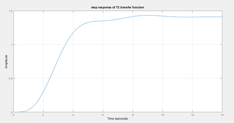
%After lot of try we can get settling time for transfer function T2 close to 7 seconds and overshoot approx 2 percent.
%T2 plot
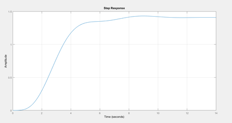
Even Tuning in automatic PID tuner it was hard to tune this….Hence best suited values are given to meet the design criterion which is often a practical case…..
Answer (b).
%in order to design the lead compensator we will use matlab tool sisotool
%write following command in MATLAb window first
clear all
s = tf(‘s’);
Gp=1/(s^4+(2*s^3)+(3.5*s^2)+(3*s))
sisotool(Gp)
% this will open a GUI window
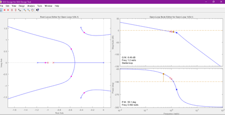
%here go to compensator window and write down the tuned values of lead compensator %as shown below
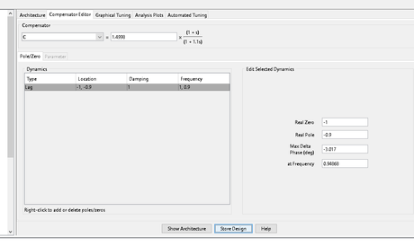
Below figure is obtained after placing suitable controller with above values as shown
Or we can write our controller as
GC_lead=1.4998*(1+s)/(1+1.1s)
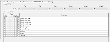
Now to see the plot go to Analysis plot window and select step response as shown
% also all the files or 18 different criteria are attached
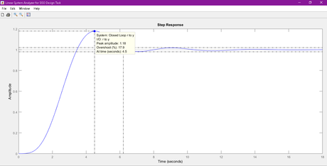
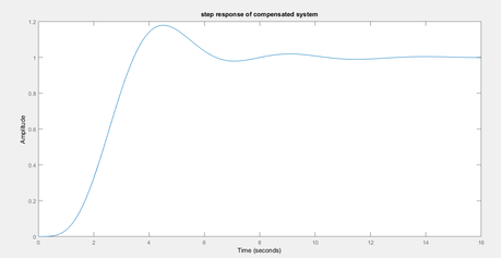
Observe the step response above we get settling time of 6.2 seconds and overshoot approx 18 %.

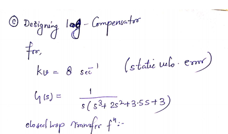
Answer ©
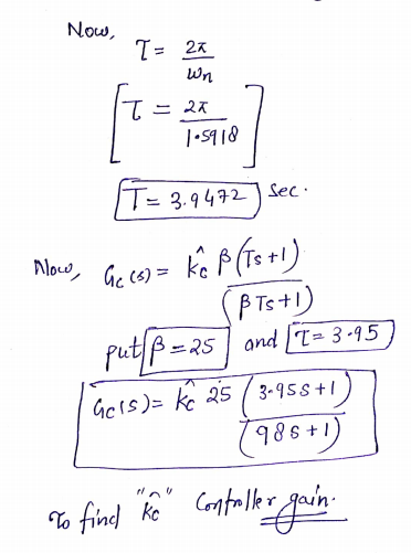
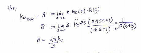
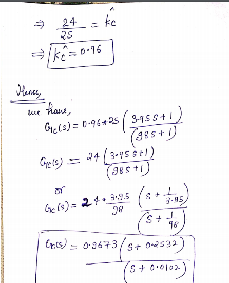
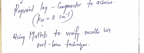
%now we will see step responses in the MATLAB for both compensated closed %loop system and uncompensated closed loop system
clc
clear all
s = tf(‘s’);
Gp=1/(s^4+(2*s^3)+(3.5*s^2)+(3*s))
uncmp_tr=Gp/(1+Gp);
Kc=0.9673;
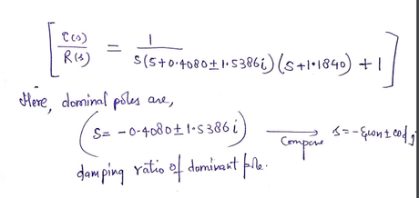
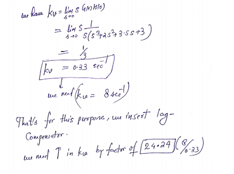
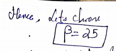
Gc=(s+0.2532)/(s+0.0102);
%closed loop transfer function
sys_comp=(Kc*Gp*Gc)/(1+(Kc*Gp*Gc))
% ***** Unit-step responses of compensated system and
% uncompensated system *****
% ***** Enter the numerators and denominators of the
% compensated and uncompensated systems *****
% ***** Specify the time range (such as t = 0:0.1:40) and enter
% step command and plot command. *****
t = 0:0.1:40;
c1 = step(uncmp_tr,t);
c2 = step(sys_comp,t);
plot(t,c1,’-‘,t,c2,’.’)
grid
text(8,0.95,’Compensated system’)
text(7,1.4,’Uncompensated system’)
title(‘Unit-Step Responses of Compensated and Uncompensated Systems’)
xlabel(‘t Sec’)
ylabel(‘Outputs c1 and c2’)
uncompensated=stepinfo(uncmp_tr)
compensated=stepinfo(sys_comp)
%Now see figure window
%See the effect of lag compensator
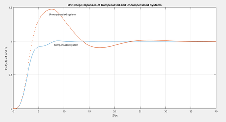
%open command window to compare important parameters of compensated and uncompensated system
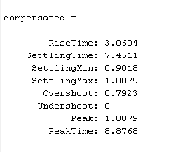
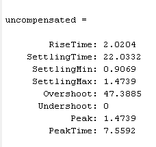
Answer (d)
For part a pid controller we got…..
Step and ramp response as shown …
%type this code for part a responses
clc
clear all
kcr=2.0199;
kp=0.6*kcr;
Ti1=7.2214;
Ti2=10.13087;
Td1=0.5554;
Td2=0.0000006777777777;
s = tf(‘s’);
Gc1=kp*(1+(1/(Ti1*s)))
Gc2=kp*(1+(1/(Ti1*s)))
Gp=1/(s^4+(2*s^3)+(3.5*s^2)+(3*s))
%closed loop transfer function
Den1=(1+(1/(Ti1*s))+(Td1*s))
Den2=(1+(1/(Ti2*s))+(Td2*s))
T1=Gc1*(Gp/(1+(Den1*Gp*kp)))
T2=Gc1*(Gp/(1+(Den2*Gp*kp)))
step(T1)
system_info_T1=stepinfo(T1)
figure
step(T2)
system_info_T2=stepinfo(T2)
grid
title(‘step response of T2 transfer function’)
figure
t=0:0.1:20
ramp=t;
[y,t]=lsim(T2,ramp,t)
plot(t,y)
grid
title(‘ramp response of T2 transfer function’)
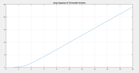
For part b lead compensator.. we got step and ramp plots as shown…
%type the code
%step and ramp response part b lead compensator
clc
clear all
s = tf(‘s’);
Gp=1/(s^4+(2*s^3)+(3.5*s^2)+(3*s))
GC_lead=1.4998*(1+s)/(1+(1.1*s))
compensated_sys=(Gp*GC_lead)/(1+(Gp*GC_lead));
figure
%step response
step(compensated_sys)
title(‘step response of compensated system’)
stepinfo(compensated_sys)
figure
t=0:0.1:20;
ramp=t;
[y,t]=lsim(compensated_sys,ramp,t);
plot(t,y)
hold on
[y,t]=lsim(Gp,ramp,t);
plot(t,y)
legend(‘compensated system’,’uncompensated system’)
grid
title(‘ramp response compensatedd and uncompensated system’)
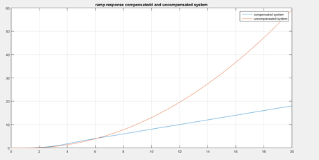
For part c lag compensator we got step and ramp plots as shown…..
%type the code to get step and ramp response
clc
clear all
s = tf(‘s’);
Gp=1/(s^4+(2*s^3)+(3.5*s^2)+(3*s))
uncmp_tr=Gp/(1+Gp);
Kc=0.9673;
Gc=(s+0.2532)/(s+0.0102);
%closed loop transfer function
sys_comp=(Kc*Gp*Gc)/(1+(Kc*Gp*Gc))
% ***** Unit-step responses of compensated system and
% uncompensated system *****
% ***** Enter the numerators and denominators of the
% compensated and uncompensated systems *****
% ***** Specify the time range (such as t = 0:0.1:40) and enter
% step command and plot command. *****
t = 0:0.1:40;
c1 = step(uncmp_tr,t);
c2 = step(sys_comp,t);
plot(t,c1,’-‘,t,c2,’.’)
grid
text(8,0.95,’Compensated system’)
text(7,1.4,’Uncompensated system’)
title(‘Unit-Step Responses of Compensated and Uncompensated Systems’)
xlabel(‘t Sec’)
ylabel(‘Outputs c1 and c2’)
figure
t=0:0.1:20;
ramp=t;
[y,t]=lsim(uncmp_tr,ramp,t);
plot(t,y)
hold on
[y,t]=lsim(sys_comp,ramp,t);
plot(t,y)
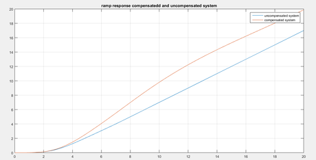
legend(‘uncompensated system’,’compensated system’)
grid
title(‘ramp response compensatedd and uncompensated system’)
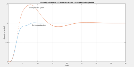
Answer (e)
See the step response from pid controller tuned after Ziegler nicolus techniques ….to avoid set kick point.

This figure is step response after tuning ko, ti and td values in MATLAB.
Also, parameters of responses are…
system_info_T2 =
RiseTime: 2.8632
SettlingTime: 7.0030
SettlingMin: 1.2791
SettlingMax: 1.4309
Overshoot: 1.9992
Undershoot: 0
Peak: 1.4309
PeakTime: 9.0263
And controller suggested after tuning is having transfer function
Gc2 =
8.752 s + 1.212
—————
7.221 s
Notice we got very low overshoot approx 2 percent but settling time is approx 7 seconds….
Similarly for lead compensator we got following results….
Controller transfer function….
GC_lead=1.4998*(1+s)/(1+1.1s)
And
Step response is having…values..
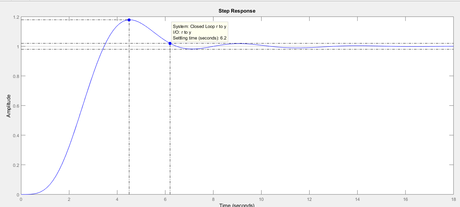
Observe the step response above we get settling time of 6.2 seconds and overshoot approx 18 %.
Hence with overall comparison we can say we got better settling time with designed lead compensator but with respact to overshoot
We have better results with pid controller.

