Tolerance, Noise and Covariation in Skilled Action

The field of motor control has been recently steadily moving towards the idea that there is no such thing as an ideal movement. The system is not trying to reliably produce a single, stable, perfect form, and movement variability has gone from being treated as noise to being studied and analysed as a key feature of a flexible, adaptive control process. This formalises Bernstein's notion of 'repetition without repetition' in movement, and recognises that the redundancy in our behavioural capabilities relative to any given task allows for multiple solutions to that task being legitimate options. 

There are many new analysis techniques within this 'motor abundance' framework, and I've reviewed most of them already; uncontrolled manifold analysis, stochastic optimal control theory and goal equivalent manifolds are the three big ones, as well as nonlinear covariation analysis. The essence of all these methods is that they take variability in the execution or outcome of a movement, and decompose that variability into variability that does not interfere with achieving the outcome and variability that does. 

This post will explain the variability decomposition process in Sternad & Cohen's (2009) Tolerance, Noise and Covariation (TNC) analysis, which my students and I are busily applying to some new throwing data from the lab. I have talked a little about this analysis here but I focused on the part of the analysis that involves a task dynamical analysis identical to the one I did for my throwing paper in 2016. In this post, I want to explain the TNC analysis itself. I will be relying on Sternad et al, 2010, which I've found to be a crystal clear explanation of the entire approach; you can also download Matlab code implementing the analysis from her website.  

Motivation

Sternad et al (2010) explain that the key motivation for developing this analysis is to remove worrying researcher degrees of freedom. UCM and the related analyses decompose variance in the kinematics of the performance of an action. There are many ways to express these kinematics; in terms of joint positions, velocities, or angles (relative or absolute). UCM gives you different answers depending on the coordinate system of the kinematic data, which makes coordinate frame a researcher degree of freedom that is rarely justified a priori. Sternad solves this by a) moving the analysis to results in execution space and b) defining that execution space a priori by a task dynamical analysis. While I think that there may be room to use UCM's coordinate sensitivity as a way to explore data for evidence of which frame of reference is behaviourally relevant, I am 100% on board with Sternad's analysis of the problem, as well as her solution. The only thing I will do here that goes beyond what she does is say that in order for the task dynamics to constrain action variability, they must be perceived. This makes behaviourally relevant task dynamics affordances (Wilson et al, 2016) and also means that the story isn't complete until we have the information analysis as well. But this task dynamical analysis is the right place to start. 

Task Dynamics of Throwing

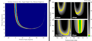
I have reviewed this specific analysis in detail here. The key is that throwing entails creating a projectile motion that either maximises distance or intercepts a distant target. For a given projectile, the dynamics of projectile motion requires three initial conditions to be specified; release angle (relative to the ground plane), release velocity (speed and direction), and release height (relative to the target height). The task dynamical analysis therefore specifies a priori that this is the execution space in which the results must be analysed. (Both Dagmar and I restricted our analysis to the 2D release angle/release speed space, because that's where most of the control action is. I did see some tentative evidence that release angle was being adaptively controlled in the 2016 paper, however, so I do want to extend this back out to the 3D execution space. I will focus here on the 2D analysis because it's way easier to graph :)Within that space of possible release parameter combinations, there is a subset that achieve the goal. For example, for a target that has some non-0 size, you can miss the center but still hit the target. This subset is referred to as the result function (bounded by lines of constant result) which maps parameter combinations onto results, and the subset of the result function that produces 0 error (e.g., exactly hits the center of the target) is the solution manifold. (Sternad notes that this function can be readily identified, but so far I've only been able to map it point by point in the simulations, rather than identify the actual function.)Figure 1 plots an example of of result functions from 2016 with one of Dagmar's; her throwing task is actually a tetherball task, so her dynamical analysis, while still projectile motion, produces a different result function to my untethered throwing task. The underlying analysis is identical, however. 

Figure 1. Result functions for two throwing tasks, plotted in execution space. Left, Wilson; Right, Sternad

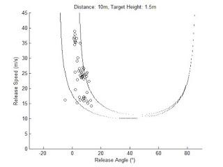
All of the following analysis evaluates the data you record from your participants relative to this solution manifold and result function. As you can see, not all regions of the space are equally useful; sometimes the result function is very narrow. But this result function gives you a reference frame to evaluate various aspects of the variability in the observed distribution of data; 

• Does it lives in the most stable region of the space (Tolerance)
• How much noise it shows (Noise)
• Does it shows evidence of a synergy in action between the execution space variables (Covariation). 

See Figure 2 for some example data from Wilson et al (2016), plotted on the appropriate result function.

Figure 2. Observed release angle/release speed combinations with the result function for that condition

Tolerance

Tolerance asks 'given the spread of data we observed, is that distributed data living in the most tolerant or error/stable region of the result function?' The analysis takes the data, preserves the spread in both dimensions, and moves that set around to all different parts of the space. It evaluates the average result of each virtual data set with respect to the result function, and the location for the data that yields the lowest distance from the solution manifold to the average result is the best location that distribution of data could hope to be centred on.  The tolerance cost is the difference between this ideal minimum and the actual location of the real data set; the smaller the tolerance cost, the more the real data is living in the most tolerant-of-error region in the space. 

Noise

Not all variability is functional; there is still good old fashioned noise in the system, specifically variation that pulls you away from the solution manifold. But how much? The analysis takes the observed data distribution, and progressively shrinks it towards the average. At each step, this average result is evaluated with respect to the result function, and the greatest improvement in performance is the Noise cost. This measures how far away from the noiseless performance the observed data are; there can still be variation in the virtual data set at this point, but by definition none of it will be moving the data out of the result function, just moving it around inside the bounds.

Covariation

In principle, the release parameters can be varied independently of each other; I can throw at (almost) any combination of release angle, speed and height within the execution space. So I could be ending up in this stable region by controlling them separately. However, I might also be taking advantage of the relationship between the variables determined by the task dynamics; I can offset speed for a higher angle, for example, because the underlying physics allows both those solutions to work. The Covariation analysis takes the original [release angle, release speed] data and shuffles the speed values so each produced speed is paired with every produced angle in a collection of virtual data sets. Each set is evaluated with respect to the result function, and the difference between the best performing virtual set and the real data set is the Covariation cost. If this is small, it tells you that the release parameter combinations that were produced were not just any old set that worked, but close to the best possible set, suggesting they were not being produced independently of each other.Note: this measure is sensitive to the coordinate frame, under certain conditions. Sternad et al (2010) propose a solution that entails rotating the coordinate frame if required, and they are working on a more robust, coordinate frame independent solution. 

Summary

Overall, each measure evaluates the observed result variability with respect to 'best case performance' defined by the task-dynamically defined result function. This quantifies the degree to which your observed data shows evidence of being organised with respect to that result function (i.e. with respect to the task dynamically defined affordance). Each of these quantifies an intuition I had about my 2016 data set; I came up with a couple of ways to assess the idea that participants were living in a nice, stable region of the space but nothing as useful as this. It is an excellent, well motivated and well executed analysis and I'm looking forward to getting into it with my current and future studies. 

References

Cohen, R., & Sternad, D. (2009). Variability in motor learning: Relocating, channeling and reducting noise. Experimental Brain Research, 193(1), 69-83.Sternad, D., Park, S.-W., Muller, H., & Hogan, N. (2010). Coordinate dependence of variability analysis. PLoS Computational Biology, 6(4), e1000751Wilson, A. D., Weightman, A., Bingham, G. P., & Zhu, Q. (2016). Using task dynamics to quantify the affordances of throwing for long distance and accuracy. Journal of Experimental Psychology: Human Perception and Performance, 42(7), 965-981.