As someone who regularly delves into human demography — often from a conservation perspective — I’m always on the lookout for quick and easy ways to get the latest and greatest datasets. Whether it’s for projection human populations, or just getting country-specific population densities, I’ve found a really nice way to interface great human data with R.

In this particular example, I’m using a api (application programming interface) key to access live data on the US Census Bureau server (don’t worry — they have global data, not just those specific to the US). What’s an ‘api key’? It’s just a code that gives you permission to access the server directly from an application via an internet link.
Step 1. Apply for an api key
This is a straightforward process and just needs to be done via this URL. The approval process doesn’t take long.
Step 2: Install the idbr package in R
This stands for the ‘(US Census Bureau) International Data Base (R)’, and grants access to and queries demographic data, including contemporary, historical, and future projections to 2100 for countries with ≥ 5000 people.
install.packages(“idbr”)
Step 3: Set api key
You need to set your user api using the following commands:
apikey <- “XXXXXXXXXXXXXXXXXXXXXXXXXXXXXXXXXXXXXXXX”
idbr::idb_api_key(apikey)
Step 4. Get data
Using the get_idb() command, you can specify all sorts of queries to get various levels of data complexity. All the variable combinations for the international database are described well here.
Example 1. Life expectancy
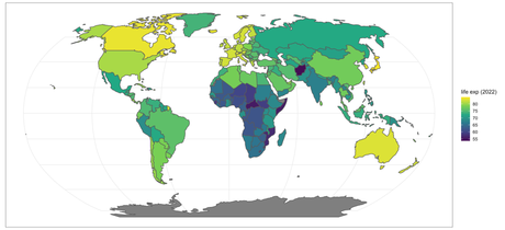
Let’s say you wanted to plot a map of the world with the shading of a country related to its average life expectancy at birth. First we get the necessary data:
lex.dat <- idbr::get_idb(
country = “all”,
year = 2022,
variables = c(“name”, “e0”),
geometry = T)
The ensuing lex.dat object looks like this:
Simple feature collection with 6 features and 4 fields
Geometry type: MULTIPOLYGON
Dimension: XY
Bounding box: xmin: -73.41544 ymin: -55.25 xmax: 75.15803 ymax: 42.68825
Geodetic CRS: SOURCECRS
code year name e0 geometry
1 AF 2022 Afghanistan 53.65 MULTIPOLYGON (((61.21082 35…
2 AO 2022 Angola 62.11 MULTIPOLYGON (((16.32653 -5…
3 AL 2022 Albania 79.47 MULTIPOLYGON (((20.59025 41…
4 AE 2022 United Arab Emirates 79.56 MULTIPOLYGON (((51.57952 24…
5 AR 2022 Argentina 78.31 MULTIPOLYGON (((-65.5 -55.2…
6 AM 2022 Armenia 76.13 MULTIPOLYGON (((43.58275 41
Here, country specifies which countries you want (in this case, all of them), year obviously specifies the relevant year, variable indicates that we want both country name and life expectancy (e0), and geometry indicates that we want spatial reference data for mapping.
Now that we’ve downloaded the data into the ‘lex.data’ object, we can plot using ggplot2:
library(ggplot2)
ggplot(lex.dat, aes(fill = e0)) +
theme_bw() +
geom_sf() +
coord_sf(cos = ‘ESRI:5403) +
scale_fill_viridis_c() +
labs(fill = “life exp (2002)”)
which gives a lovely plot of life expectancy at birth by country following the viridis color scheme:

(note: the options stated in the ggplot code above relate to different coordinate and display options; see theme_bw, geom_sf, coord_sf).
Example 2. Population density
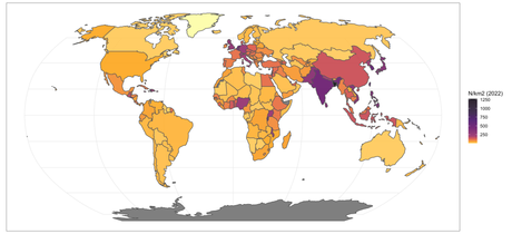
Let’s say you wanted to plot the population density of all countries in the world on a map. As above, the first step is to acquire the relevant data:
popD.dat <- idbr::get_idb(
country = “all”,
year = 2022,
variables = c(“name”, “POP”, “AREA_KM2”),
geometry = T)
popD.dat$popD <- popD.dat$pop / popD.dat$area_km2
valrange <- rescale(unique(c(seq(0,1,0.1), seq(1,200,5),
seq(200, 400, 20), seq(400, 800, 30), seq(800,
max(popD.dat$popD, na.rm=T), 40)), to=c(0,1)))
ggplot(popD.dat, aes(fill = popD)) +
theme_bw() +
geom_sf() +
coord_sf(cos = ‘ESRI:5403) +
scale_fill_viridis_c(direction=-1, option=”B”,
alpha=0.9, values=valrange) +
labs(fill = “N/km2 (2002)”)
Here, the valrange object sets a non-uniform shading to take into account the log-linear nature of the density data.

Of course, there a thousands of possible combinations to play with, so have fun!

