How to Create an Image of a Pie Chart in Excel to Use for Your Blog

Using visuals such as charts and graphs to help illustrate the trends or meanings behind data is a common practice among blog writers. Pie charts are often used to depict the proportions of categories in relation to the whole by dividing a circle (or pie) into sectors. For example, a pie chart of social media followers could be divided into each social media platform to see the impact that each platform has overall and where a marketing strategy would be most successful.

Creating the Chart:

1. Create the worksheet in Excel by opening a new workbook or adding a new Worksheet to an existing workbook by clicking a new Tab at the bottom.
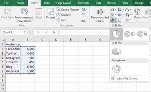
2. Highlight the data you would like included in the Pie Chart.
   
3. Click the Insert Tab in the Ribbon. In the charts box, Select the Pie Chart and choose the style you prefer.
4. Once the Chart is created within Excel be sure to make any adjustments necessary.
   • Change the Title of the chart by double-clicking Chart Title and entering in the Title of your choice.
     
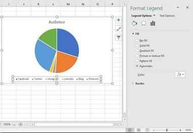
   • Clicking on the chart itself will open a new Tab in the Ribbon for Chart Tools. Under Design you can choose the style, add elements, or change the color scheme. The Format Tab allows you to change the lines, text, numbers, add shapes or change sizes.
   • To change the characteristics of the chart, double-click anywhere on the chart to open the Formatting dialog box. Here you can make changes to the legend or any of the changes you could complete within the Chart Tools Tab.
     
5. Once all Formatting is complete and the Pie Chart looks exactly how you want it you can turn the Chart into an Image.

Creating an Image:

Copy and Paste method:

1. Select the chart and hit Ctrl + C or right click and select Copy.
2. Open a different Microsoft Office file, Word or Power Point for example, right-click and select Paste as Picture.
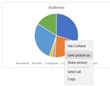
3. Right-Click on the Chart one more time and select Save Picture As.
   
4. Select the file type you would like, be it Jpeg or PNG, name the file and hit OK.

Note: This method also works by Pasting the Chart into any photo editing software or into Paint. Also, when pasting the Chart into Power Point there is no need to paste the chart as a Picture.

Saving multiple charts as images:

If your workbook or worksheet has multiple charts that you wish to save as images you could go through and use the Copy and Paste method for each individual chart or you can save the entire workbook as a webpage to quickly save all charts.

1. Go to the File Tab in the Ribbon and select Save As.
2. Choose Webpage as the File Type
3. Choose the folder you wish to save the file to and click Save.
4. Open the newly save Webpage File.
   
5. Right-click each Chart and choose Save Picture As to separate each Chart as a picture that can easily be inserted into your blog.

Congratulations; you’ve now made a beautiful pie chart you can use for your own purposes.