Microsoft Office is one of the widely used (if not the popular) office suite available today. And, Excel is their spreadsheet software we get along with other tools in the MS Office package.
I hope you know there are some formulas and shortcuts available in Excel using which, you can make the tabulation effortless.
Today, I am going to walk you through some methods to alphabetize in Excel. Trust me; you will thank me later for this!
How to Alphabetize in Excel?
Before getting deep into the core of this post, you must know what the term ‘alphabetization’ in Excel means.
What is Alphabetization in Excel?
Have you heard of sorting? Alphabetization is more of a type of sorting in Excel. Here, you will sort available data in alphabetical (A to Z) or reverse-alphabetical (Z to A) order. If you have a lot of numbers to present, you should present that data in Charts. Here is how you can create charts in Excel.
That’s all. I hope you know what alphabetization means now.
Uses of Alphabetization
#1. Alphabetization makes the data in a spreadsheet more sensible and easy to search for a particular item.
#2. After alphabetization, the duplicate data can be identified without sweating.
How to Alphabetize in Excel?
Now we are here, in the central section of this post. You are going to learn how the alphabetization can be done in Excel.
Method 1: Quick Alphabetization with Buttons
Follow the steps given below to sort columns in Excel.
Step 1: Open the Excel file you want to sort or alphabetize. You can either double-click on the file or use the open option within Excel. If you go with the latter, you should browse the file in which the alphabetization of data is needed.
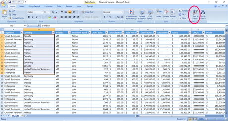
Step 2: As we are using Excel sort by column, you have to select the column containing the data for alphabetization. The selection of an entire column is done easily by a single click on the letter label (A, B, C, etc. ) of the column.

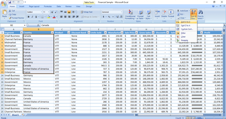
Step 3: Now, you must look at the ribbon-like menu with a set of buttons. There, you can see a button with a funnel, A and Z with name Sort and Filter. Click on to see a new menu with a bunch of new options.

Step 4: You will see four options there; Sort A to Z, Sort Z to A, Custom Sor, and Filter. The first choice is for proper alphabetical order and the second for reverse alphabetical order. The third, Custom Sort needs you to make a few setups.
As we are quickly sorting data here, you need to choose either A to Z or Z to A. If you have something really confidential, it is always a good idea to hide the columns in excel.
Now you can see that all the data are sorted. Though I explained the process in four steps, you
Method 1: Using Custom Sort
Here, you will have to do a few steps more as compared to the previous method.
Step 1: You have to make the necessary selections first. I recommend selecting the entire table so that, sorting based on site headers will be easier.
Step 2: Click on the Sort& Filter button. (If you don’t find the ribbon-like bar with the buttons, consider reading the next section).
Step 3: The third option just above Filter (Custom Sort) is the one we need here. So click on Custom Sort option.
Also Read:- How to Hide Columns in Excel?
Step 4: Now, you will see a new dialog box (check the image down below to get an idea of it). Under column, you can spot a Sort by option. In order to sort columns in Excel, you must adjust the option.

Clicking on the drop-down menu just right to the Sort by option reveals the column headers. That particular option determines on the basis of which column; the data should be sorted or alphabetized.
So, you should choose one column header.
Step 5: If your Excel sheet lacks headers, uncheck ‘My data has headers’. Don’t miss this step because Excel will not sort the first row if you uncheck this one.
Step 6: By default, the selection under Sort on the option is Value. If you find anything else, don’t forget to change the same to Value.
Step 7: Next option is Order. As you are going to alphabetize data in Excel, you don’t need a lot of orders but two; A to Z and Z to A.
Clicking on the Order drop-down menu gives you both the alphabetization options. Choose one that suits you the best.
Step 7: Finally, hit the OK button to finish the process.
What if You Don’t Find Sort& Filter Button in Excel?
The situations are rare when you can’t find Sort& Filter button. If you are in such a situation, check the Data tab. There, you can find alphabetization and custom sort buttons separately.

If the above solution doesn’t rescue you, go to View tab and click on Menu bars. There, you can find some checkboxes. Enable Standard from the menu bar options.
Method 3: Using Shortcuts
I know you are familiar with computer shortcuts, aren’t you? Shortcuts are time savers for those who use it efficiently.
Three keyboard shortcuts are available which can assist you in sorting Excel data within no time.
Alt+ H, S, S – For alphabetical sorting
Alt+ H, S, O – For reverse-alphabetical sorting
Alt+ D, S – To open Custom Sort dialog box
N.B. – Don’t forget to select the necessary columns before hitting the shortcut keys. In earlier versions of Office, A to Z and Z to A quick sorting only arrange the selected columns. So, you must select the entire table in order to sort all the cells.
Also Read:- How to Create a Pie Chart in Excel?
Wrapping Up
Don’t you know how to alphabetize in Excel? I have explained three different methods for sorting.
In addition to all the above methods to sort columns in Excel, you can make use of VLOOKUP and COUNTIF statements as well. Also, learn to create bar graphs in excel.
We already have a VLOOKUP Excel tutorial here on ExpertHoot. You should check out the same for basic information.
If you face any difficulty in sorting data, don’t forget to let us know using the comment section down below.
And, have a second to hit one of the share buttons to help your needy social media friends.

