The other day I was tasked with revising a figure for a paper (that should be out soon) where I had to figure out how to compare incident times in a biologically meaningful way.

Without giving away too many details, we had a long list of incidents spread right across Australia, covering all periods of the year and going back to the early 20th Century. The specifics of the ‘incidents’ isn’t important here — suffice it to say they were biological in nature, and we wanted to see if they were clustered around any particular times of the day.
Yes, we could just do a histogram of the time bins (say, every 2 hours), but this ignores a very important phenomenon — 17:00 in July in Hobart isn’t directly comparable to 17:00 in January in Darwin (and so on). What matters instead — from a biological/phenological perspective — is the period of day in terms of available light.
Fortunately, there are some clear definitions of relative light availability we can use.
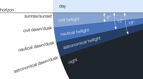
‘Night’ is defined as the time between astronomical dusk and astronomical dawn, which are when the sun is 18º below the horizon. ‘Twilight’ is the period between night and sunrise/sunset (the latter being when the sun first appears/disappears above/below the horizon), further broken down into three periods: astronomical twilight, nautical twilight, and civil twilight. These latter refer to when the sun is 18º, 12º, and 6º below the horizon, respectively.

It’s still ‘dark’ in astronomical twilight, but light starts to be discernible at the start of nautical twilight. We can therefore define four major periods of relative light availability per 24-hour period: night (between the start of astronomical dusk and end of astronomical dawn), dawn (between the end of nautical twilight and sunrise), day (between sunrise and sunset), and dusk (between sunset and the onset of astronomical twilight).
Phew!
So, after all that malarkey, now we need a way of determining when those transition periods occur on any given day in any given location. Sounds difficult, but, there’s a function for that!
R comes to the rescue here with two cool packages: suncalc gives you these transitions for any given latitude/longitude coordinate, and lutz gives you the time zone for coordinate. The latter is needed for the former. Here are the steps:
Step 1.
Let’s say you have a location (we’ll use my home city of Adelaide at latitude = -34.945989, longitude = 138.533281; this is the airport), a date (we’ll say 16 July 1972 just for the hell of it), and a time (17:09). Obviously, this time could not be dawn, but it could conceivably be day, dusk, or even night.
Step 2.
Install the packages in R:
install.packages(“suncalc”, “lutz”)
Step 3.
Create a coordinate vector:
coords <- c(-34.945989, 138.533281)
Step 4.
Figure out what time zone relates to these coordinates:
timezone <- tz_lookup_coords(coords[1], coords[2], method = “accurate”)
Step 5.
Combine the date and time into a single date-time POSIX object:
A little trick first. I often come across times in databases that are entered as 24-hour numerics; for example, 06:02 (morning) is entered as 602 (i.e., the leading zero is dropped). I need to get this into a time format, so I use sprintf to do this:
time.num <- 1709
time24 <- sprintf(“%04d”, time.num) # makes sure there are four digits
hr24 <- substr(time24, 1, 2) # carves off the hour
mn60 <- substr(time24, 3, 4) # carves off the minutes
Now, we need to get the date itself into the right format:
date.char <- “16-07-1972” # DD-MM-YYYY
and then combine the date and time:
datetime <- strptime(paste(date.char, ” “, hr24,”:”, mn60, sep=””), format=”%d-%m-%Y %H:%M”)
Step 6.
Now it’s as easy as invoking the getSunlightTimes function in the suncalc package to get the sunlight transition periods:
sunlight.times <- getSunlightTimes(date=as.Date(datetime), lat=coords[1], lon=coords[2], tz=timezone)
Note that this also accounts for daylight savings!
From this we can calculate dawn, day, dusk, and night periods to determine in which our time of 17:09 falls:
dawn <- c(strftime(sunlight.times$dawn, format=”%H:%M”), strftime(sunlight.times$sunrise, format=”%H:%M”))
day <- c(strftime(sunlight.times$sunrise, format=”%H:%M”), strftime(sunlight.times$sunset, format=”%H:%M”))
dusk <- c(strftime(sunlight.times$sunset, format=”%H:%M”), strftime(sunlight.times$night, format=”%H:%M”))
night <- c(strftime(sunlight.times$night, format=”%H:%M”), strftime(sunlight.times$dawn, format=”%H:%M”))
So, on 16 July 1972, dusk was from 06:54−07:21, day was 07:21−17:24, dusk was 17:24−18:53, and night was 18:53−06:54. This means that our time of 17:09 was still considered day, but only just.
If you want to see a more comprehensive example of this, check out this repository in Github.

